

Imbalanced Domain Learning
Fraud Detection Course - 2020/2021
Nuno Moniz
nuno.moniz@fc.up.pt
Today
- Beyond Standard ML
- Imbalanced Domain Learning
- 2.1 Problem Formulation
- 2.2 Evaluation/Learning
- Strategies for Imbalanced Domain Learning
- Practical Examples
Beyond Standard Machine Learning


Famous ML Mistakes #1

Famous ML Mistakes #2

Machine Learning, Predictive Modelling
- The goal of predictive modelling is to obtain a good approximation for an unknown function
- \(Y = f(x_1, x_2,\cdots)\)
- What you need (the most basic):
- A dataset
- A target variable
- Learning algorithm(s)
- Evaluation metric(s)
Modelling Wally
- Your task is to find Wally among 100 people
- You train two models using the state-of-the-art in Deep Learning
- Model 1 obtains 99% Accuracy
- Model 2 obtains 1% Accuracy
- Confusion Matrix?

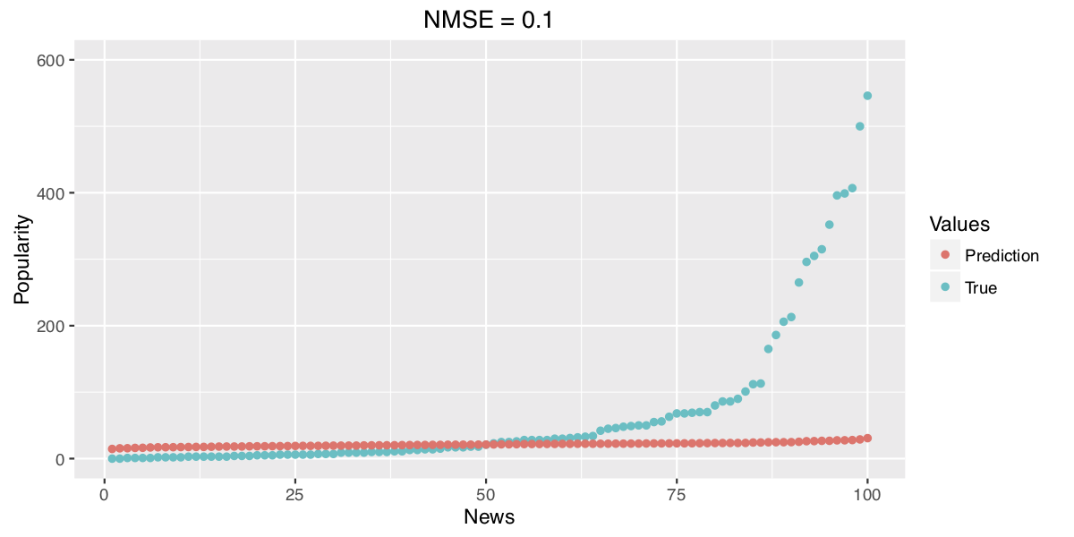
Predicting Popular News
- Your task is to anticipate the most popular news of the day
- You train two models using the state-of-the-art Ensemble Learning techniques
- Model 1 obtains 0.1 NMSE
- Model 2 obtains 0.5 NMSE
- Normalized Mean Squared Error: \(\frac{1}{n} \sum_{i=1}^{n} \frac{(\hat{y_i} - y_i)^2}{y_i^2}\)
Imbalanced Domain Learning
Imbalanced Domain Learning?
- It's still predictive modelling, and as such...
- "The goal of predictive modelling is to obtain a good approximation for an unknown function"
- \(Y = f(x_1, x_2,\cdots)\)
- Standard predictive modelling has some assumptions:
- The distribution of the target variable is balanced
- Users have uniform preferences: all errors were born equal
- Assumptions in Imbalanced Domain Learning:
- The distribution of the target variable is imbalanced
- Users have non-uniform preferences: some cases are more important
- The more important/relevant cases are those which are rare or extreme
Imbalanced Domain Learning - Nominal Target
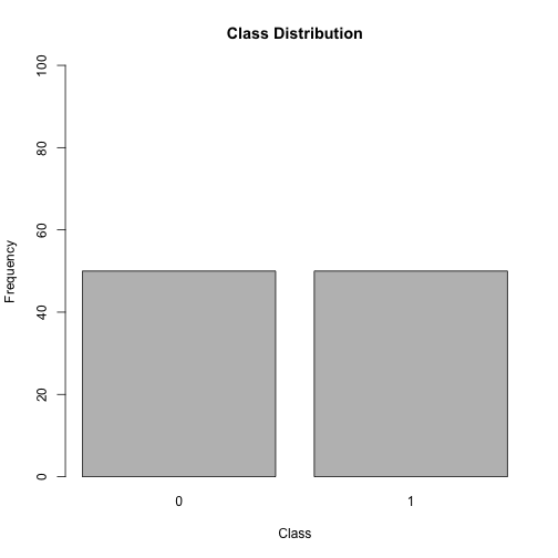 A balanced distribution
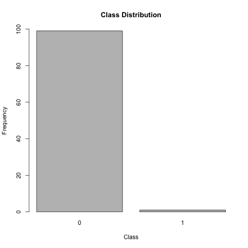 An imbalanced distribution
Imbalanced Domain Learning - Numerical Target
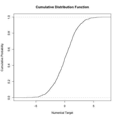 A balanced distribution
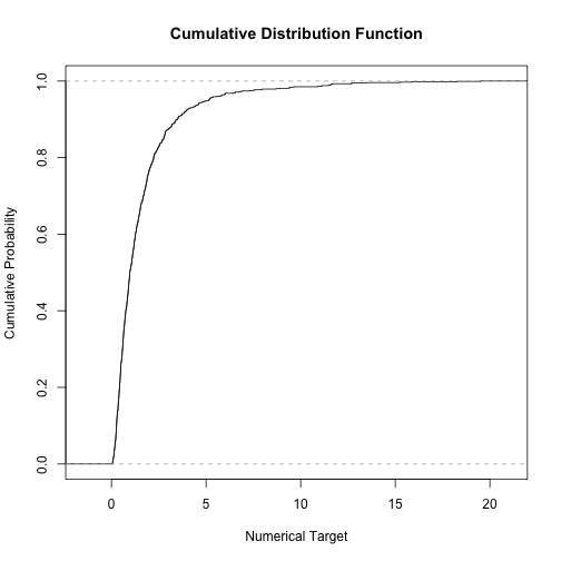 An imbalanced distribution
Problems with Imbalanced Domains
There are two main problems when learning with imbalanced domains
1. How to learn?
2. How to evaluate?
How to learn?
- Models are optimized to accurately represent the maximum of information
- When there's information imbalance, this means that it will more likely represent the majority type of information in detriment to the minority (rare/extreme cases)
How to evaluate?
- Most of the most well-known evaluation metrics are focused on assessing the average behaviour of the models
- However, there are a lot of cases where the evaluation objective is to understand if a model is capable of predicting a certain class or subset of values, i.e. imbalanced domain learning
The Problem of Evaluation
- This problem is different for classification and regression tasks
- Imbalanced Learning has been explored in classification for over 20 years, but in regression problems it is very recent
- The main idea is this: for evaluating this type of problems:
- Remember that not all cases are equal
- You're focused on the ability of models in predicting a rare cases
- Missing a prediction of rare cases is worst than missing a normal case
The Problem of Evaluation
Classification
Standard Evaluation
- Accuracy
- Error Rate (complement)
Non-Standard Evaluation
- F-Score
- G-Mean
- ROC Curves / AUC
Regression
Standard Evaluation
- MSE
- RMSE
Non-Standard Evaluation
- MSE\(_\phi\)
- RMSE\(_\phi\)
- Utility-Based Metrics (
UBLR Package)
The Problem of Learning
Imagine the following scenario:
- You have a dataset of 10,000 cases of credit transactions classified as
FraudorNormal - This dataset has 9,990 cases classified as
Normal, and only 10 cases classified asFraud - Learning algorithm are not human beings: they're programmed to operate in a pre-determined way
- This usually means that the problem they want to solve is: how can we accurately represent the data?
However, learning algorithms make choices - they have assumptions.
The most hazardous for imbalanced domain learning are:
- Assuming that all cases are equal
- Internal optimization/decisions based on standard metrics
The Problem of Learning
Instead of "It's all about the bass", it's in fact all about the mean/mode.
Remember this?


Until now
- There's more to machine learning than standard tasks
- Learning algorithms are biased and,
- Algorithms are focused on reducing the average error/representing the majority cases
- Beware of standard evaluation metrics if your task is imbalanced domain learning
Strategies for Imbalanced Domain Learning
Strategies for Imbalanced Domain Learning
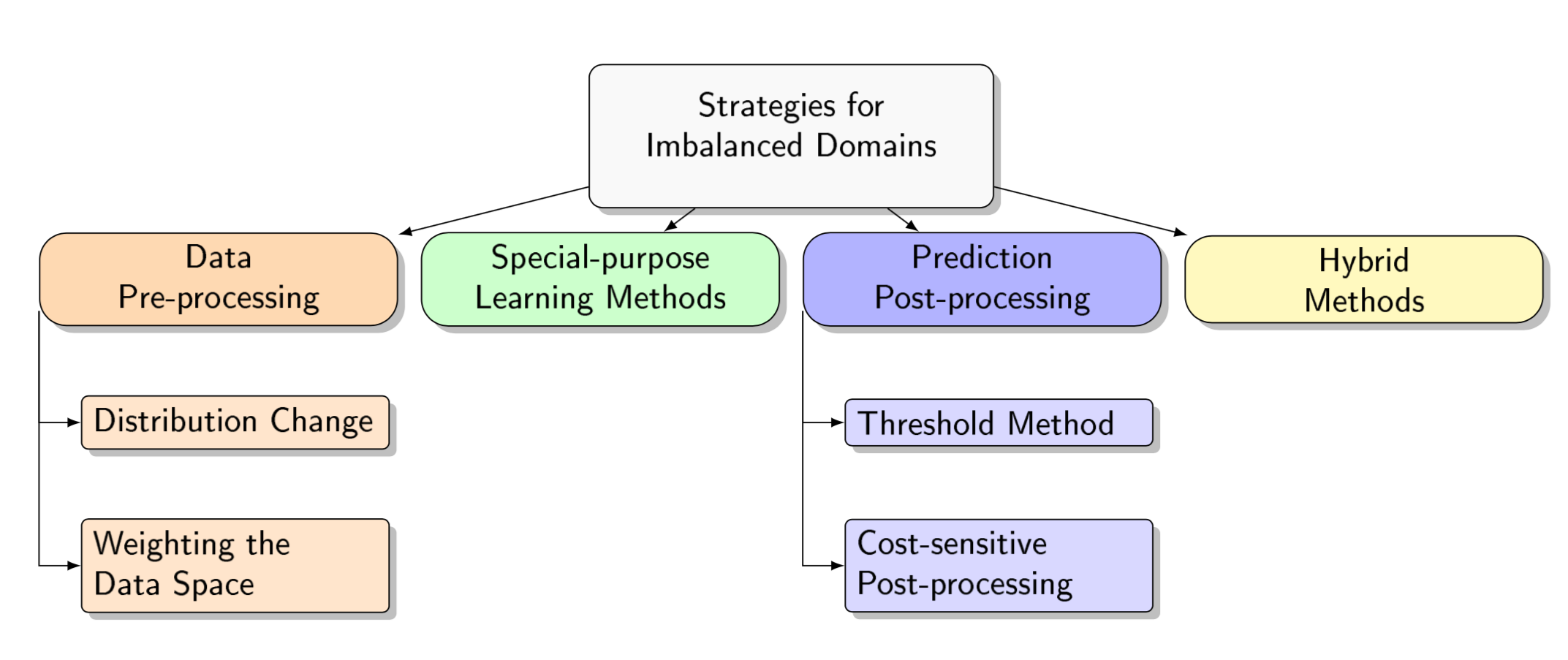
Data Pre-Processing
- Goal: change the examples distribution before applying any learning algorithm
- Advantages: any standard learning algorithm can then be used
- Disadvantages
- difficult to decide the optimal distribution (a perfect balance does not always provide the optimal results)
- the strategies applied may severly increase/decrease the total number of examples


Special-purpose Learning Methods
- Goal: change existing algorithms to provide a better fit to the imbalanced distribution
- Advantages
- very effective in the contexts for which they were design
- more comprehensible to the user
- Disadvantages
- difficult task because it requires a deep knowledge of both the algorithm and the domain
- difficulty of using an already adapted method in a different learning system

Prediction Post-Processing
- Goal: change the predictions after applying any learning algorithm
- Advantages: any standard learning algorithm can be used
- Disadvantages: potential loss of models interpretability

Practical Examples
Practical Examples - Data Pre-Processing
- Data Pre-Processing strategies are also known are Resampling Strategies
- These are the most common strategies to tackle imbalanced domain learning tasks
- We will look at practical examples for both classification and regression using:
- Random Undersampling
- Random Oversampling
- SMOTE
Preliminaries in R
- Install the package
UBLfrom CRAN
install.packages("UBL")
- Install
UBLfrom GitHub
library(devtools)
# stable release
install_github("paobranco/UBL",ref="master")
# development release
install_github("paobranco/UBL",ref="develop")
- After installation, the package can be used, as any other R package
library(UBL)
Data for Pratical Examples - Classification Tasks
- We will use the well-known dataset
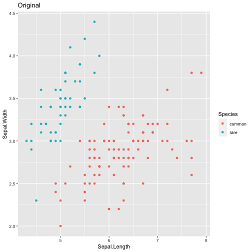
iris. The iris flower data set or Fisher's Iris data set is a multivariate data set introduced by the British statistician and biologist Ronald Fisher in 1936 - The data set consists of 50 samples from each of three species of Iris (Iris setosa, Iris virginica and Iris versicolor).
- For the purpose of the practical examples, we will consider the class
setosaas being the rare class, and the other classes as being the normal class
library(UBL)
# generating an artificially imbalanced data set
data(iris)
data <- iris[, c(1, 2, 5)]
data$Species <- factor(ifelse(data$Species == "setosa","rare","common"))
## checking the class distribution of this artificial data set
table(data$Species)
##
## common   rare
##    100     50
Random Undersampling
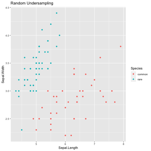
- To force the models to focus on the most important and least represented class(es) this technique randomly removes examples from the most represented and therefore less important class(es)
- As such, the modified data set obtained is smaller than the original one
- The user must always be aware that to obtain a more balanced data set, this strategy may discard useful data
- Therefore, this strategy should be applied with caution, specially in smaller datasets

Random Undersampling
# using a percentage provided by the user to perform undersampling
datU <- RandUnderClassif(Species ~ ., data, C.perc = list(common=0.4))
table(datU$Species)
##
## common   rare
##     40     50
# automaticaly balancing the data distribution
datB <- RandUnderClassif(Species ~ ., data, C.perc = "balance")
table(datB$Species)
##
## common   rare
##     50     50
Random Undersampling
Random Oversampling
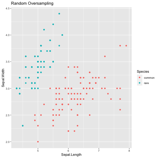
- This strategy introduces replicas of randomly selected examples from relevant classes of the data set, e.g. replicating fraud cases
- This allows to obtain a better balanced data set without discarding any important examples
- However, this method is highly prone to over-fitting (think a data set only with red apples)
- This methods also has a strong impact on the number of examples of the new data set which can be a difficulty for the algorithm

Random Oversampling
 # using a percentage provided by the user to perform oversampling
datO <- RandOverClassif(Species ~ ., data, C.perc = list(rare=3))
table(datO$Species)
##
## common   rare
##    100    150
# automaticaly balancing the data distribution
datB <- RandOverClassif(Species ~ ., data, C.perc = "balance")
table(datB$Species)
##
## common   rare
##    100    100
Random Oversampling

SMOTE
- Synthetic Minority Over-Sampling Technique
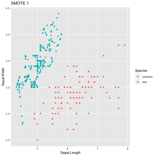
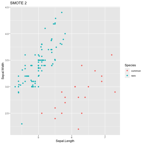
- The SMOTE algorithm is a strategy that performs oversampling via the generation of synthetic examples
- A synthetic case of the minority class is generated via the interpolation of two minority class cases
- A new minority case example is obtained with a seed example from that class and one of its randomly selected \(k\) nearest neighbours
- With two examples, a new synthetic case is obtained by interpolating the example features
SMOTE
 #using smote just to oversample the class rare
datSM1 <- SmoteClassif(Species ~ ., data, C.perc = list(common=1,rare=6))
table(datSM1$Species)
##
## common   rare
##    100    300
# user defined percentages for both undersample and oversample
datSM2 <- SmoteClassif(Species~., data, C.perc=list(common=0.2, rare=2))
table(datSM2$Species)
##
## common   rare
##     20    100
SMOTE

SMOTE

Data for Pratical Examples - Regression Tasks
- We will use the
algaedata set from the packageDMwR - This data set contains observations on 11 variables as well as the concentration levels of 7 harmful algae. Values were measured in several European rivers
- We will focus on the target variable
a7
# loading the algae data set
library("DMwR")
## Error in library("DMwR"): there is no package called 'DMwR'
data(algae)
algae <- knnImputation(algae)
## Error in knnImputation(algae): could not find function "knnImputation"
# checking the density distribution of the data set
plot(density(algae$a7))
## Error in density(algae$a7): object 'algae' not found
Extreme Values?
- In classification tasks, it is easy to know if a distribution is imbalanced: class frequency
- How can we do it regression tasks?
- Specifically, how can we determine the importance (or relevance) of a given value in a domain?
- Which values should be considered extreme?
Relevance Functions
- When dealing with imbalanced regression tasks the user should specify which are the important values
- However, this can be a very difficult task: continuous domains are potentially infinite
- Professor Rita Ribeiro (Ribeiro, 2011) proposed a framework for defining relevance functions of a given continuous target variable. This framework:
- Includes an automatic method that allows to obtain a relevance function from the target value distribution. It is based on boxplot rules (lookup adjusted boxplot). This method assumes that the most important values for users are those considered as extreme by such rules
- It also allows users to manually specify the values which are considered to be relevant and irrelevant using a matrix (the user inserts a given set of points, and the remaining are interpolated)
Ribeiro, R. Utility-based regression. Diss. PhD thesis, Dep. Computer Science, Faculty of Sciences-University of Porto, 2011
Relevance Threshold
- After obtaining a relevance function for a given target variable, we still have to define which range of relevance values should be considered as being the most important values
## Error in adjbox(algae$a7, horizontal = TRUE): object 'algae' not found
## Error in library(IRon): there is no package called 'IRon'
## Error in loadNamespace(name): there is no package called 'IRon'
Random Undersampling
- The Random Undersampling approach is simply based on the random removal of examples from the original data set
- The examples removed are randomly selected from the subset of examples with less important ranges of the target variable, those with a relevance that is below the user-defined threshold
- You need to define a relevance function, a relevance threshold and the percentage of undersampling to perform
# using the automatic method for defining the relevance function and the default threshold (0.5)
Alg.U <- RandUnderRegress(a7 ~ ., algae, C.perc = list(0.5)) # 50% undersample
## Error in which(names(dat) == as.character(form[[2]])): object 'algae' not found
Alg.UBal <- RandUnderRegress(a7 ~ ., algae, C.perc = "balance")
## Error in which(names(dat) == as.character(form[[2]])): object 'algae' not found
Random Undersampling
## Error in density(algae$a7): object 'algae' not found
## Error in density(Alg.U$a7): object 'Alg.U' not found
## Error in density(algae$a7): object 'algae' not found
## Error in density(Alg.UBal$a7): object 'Alg.UBal' not found
Random Oversampling
- The Random Oversampling approach is simply based on the introduction of random copies of examples from the training data set
- These replicas are only introduced in the most important ranges of the target variable, i.e. for cases with a relevance value that is above the user-defined threshold
- It is necessary to define a relevance function, a relevance threshold and the percentage of oversampling to perform
# using the automatic method for defining the relevance function and the default threshold (0.5)
Alg.O <- RandOverRegress(a7 ~ ., algae, C.perc = list(4.5))
## Error in which(names(dat) == as.character(form[[2]])): object 'algae' not found
Alg.OBal <- RandOverRegress(a7 ~ ., algae, C.perc = "balance")
## Error in which(names(dat) == as.character(form[[2]])): object 'algae' not found
Random Oversampling
## Error in density(algae$a7): object 'algae' not found
## Error in density(Alg.U$a7): object 'Alg.U' not found
## Error in density(Alg.O$a7): object 'Alg.O' not found
## Error in density(algae$a7): object 'algae' not found
## Error in density(Alg.UBal$a7): object 'Alg.UBal' not found
## Error in density(Alg.OBal$a7): object 'Alg.OBal' not found
SMOTE
- The relevance function and the relevance threshold defined determine which are the relevant and non-relevant (normal) cases
- This algorithm combines an oversampling strategy by interpolation of important examples with a random undersampling approach
- The procedure is in all similar to the generation of synthetic examples in SMOTE for classification tasks
# we have two bumps: the first must be undersampled and the second oversampled.
# Thus, we can chose the following percentages:
thr.rel=0.8; C.perc=list(0.2, 4)
## Error in knnImputation(algae): could not find function "knnImputation"
# using these percentages and the relevance threshold of 0.8 with all the other parameters default values
Alg.SM <- SmoteRegress(a7 ~ ., algae, thr.rel = thr.rel, C.perc = C.perc, dist = "HEOM")
## Error in SmoteRegress(a7 ~ ., algae, thr.rel = thr.rel, C.perc = C.perc, : object 'algae' not found
# use the automatic method for obtaining a balanced data set
Alg.SMBal <- SmoteRegress(a7 ~ ., algae, thr.rel = thr.rel, C.perc = "balance", dist = "HEOM")
## Error in SmoteRegress(a7 ~ ., algae, thr.rel = thr.rel, C.perc = "balance", : object 'algae' not found
SMOTE
## Error in density(algae$a7): object 'algae' not found
## Error in density(Alg.U$a7): object 'Alg.U' not found
## Error in density(Alg.O$a7): object 'Alg.O' not found
## Error in density(Alg.SM$a7): object 'Alg.SM' not found
## Error in density(algae$a7): object 'algae' not found
## Error in density(Alg.UBal$a7): object 'Alg.UBal' not found
## Error in density(Alg.OBal$a7): object 'Alg.OBal' not found
## Error in density(Alg.SMBal$a7): object 'Alg.SMBal' not found
Wrap-up
Summary
1. Machine Learning has a lot of faces and some of them are not pretty
Imbalanced Domain Learning is considered one of the most important topics for Machine Learning and Data Mining
There are a lot of strategies to tackle this type of tasks, but all of them have their advantages and disadvantages
Solutions are domain-dependent
Remember: before you begin tackling any ML problem, investigate the domain and your objective.
Three Challenges for the Future
1. Auto-Machine Learning and Imbalanced Domain Learning
Targeted Resampling: reduce the variance of outcomes in strategies
How to "force" a model to account for small concepts without sampling
