
Predictive Modelling 1
Fraud Detection Course - 2020/2021
Nuno Moniz
nuno.moniz@fc.up.pt
Today
- Introduction to Predictive Modelling
- 1.1. Evaluation Metrics
- Tree-based Models
- Naïve Bayes
Introduction to Predictive Modelling
Introduction to Predictive Modelling
Prediction is:
the ability to anticipate the future (forecasting).
possible if we assume that there is some regularity in what we observe, i.e. if the observed events are not random.
Example: Medical Diagnosis
Given an historical record containing the symptoms observed in several patients and the respective diagnosis, try to forecast the correct diagnosis for a new patient for which we know the symptoms.
Prediction Models
- Are obtained on the basis of the assumption that there is an unknown mechanism that maps the characteristics of the observations into conclusions/diagnoses. The goal of prediction models is to discover this mechanism.
- Going back to the medical diagnosis what we want is to know how symptoms influence the diagnosis.
- Have access to a data set with “examples” of this mapping, e.g. this patient had symptoms \(x\), \(y\), \(z\) and the conclusion was that he had disease \(p\)
- Try to obtain, using the available data, an approximation of the unknown function that maps the observation descriptors into the conclusions, i.e. \(Prediction = f(Descriptors)\)
“Entities” involved in Predictive Modelling
- Descriptors of the observation: set of variables that describe the properties (features, attributes) of the cases in the data set
- Target variable: what we want to predict/conclude regards the observations
- The goal is to obtain an approximation of the function \(Y = f(X_1, X_2, \cdots, X_p)\), where \(Y\) is the target variable and \(X_1\), \(X_2\), \(\cdots\), \(X_p\) the variables describing the characteristics of the cases.
- It is assumed that \(Y\) is a variable whose values depend on the values of the variables which describe the cases. We just do not know how!
- The goal of the modelling techniques is thus to obtain a good approximation of the unknown function \(f()\)
How are the Models Used?
Predictive models have two main uses:
- Prediction: use the obtained models to make predictions regards the target variable of new cases given their descriptors.
- Comprehensibility: use the models to better understand which are the factors that influence the conclusions.
Types of Prediction Problems
- Depending on the type of the target variable \(Y\) we may be facing two different types of prediction models:
- Classification Problems: the target variable \(Y\) is nominal, e.g. medical diagnosis - given the symptoms of a patient try to predict the diagnosis
- Regression Problems: the target variable \(Y\) is numeric e.g. forecast the market value of a certain asset given its characteristics
Examples of Prediction Problems
Classification Task
\(Species = f(Sepal.Width, \cdots)\)
##   Sepal.Width Petal.Length Petal.Width Species
## 1         3.5          1.4         0.2  setosa
## 2         3.0          1.4         0.2  setosa
## 3         3.2          1.3         0.2  setosa
## 4         3.1          1.5         0.2  setosa
## 5         3.6          1.4         0.2  setosa
## 6         3.9          1.7         0.4  setosa
Regression Task
\(a1 = f(Cl, \cdots)\)
##       Cl    NO3     NH4    oPO4     PO4 Chla   a1
## 1 60.800  6.238 578.000 105.000 170.000 50.0  0.0
## 2 57.750  1.288 370.000 428.750 558.750  1.3  1.4
## 3 40.020  5.330 346.667 125.667 187.057 15.6  3.3
## 4 77.364  2.302  98.182  61.182 138.700  1.4  3.1
## 5 55.350 10.416 233.700  58.222  97.580 10.5  9.2
## 6 65.750  9.248 430.000  18.250  56.667 28.4 15.1
Types of Prediction Models
- There are many techniques that can be used to obtain prediction models based on a data set.
- Independently of the pros and cons of each alternative, all have some key characteristics:
- They assume a certain functional form for the unknown function \(f()\)
- Given this assumed form the methods try to obtain the best possible model based on:
- the given data set
- a certain preference criterion that allows comparing the different alternative model variants
Functional Forms of the Models
- There are many variants. Examples include:
- Mathematical formulae - e.g. linear discriminants
- Logical approaches - e.g. classification or regression trees, rules
- Probabilistic approaches - e.g. naive Bayes
- Other approaches - e.g. neural networks, SVMs, etc.
- Sets of models (ensembles) - e.g. random forests, adaBoost
- These different approaches entail different compromises in terms of:
- Assumptions on the unknown form of dependency between the target and the predictors
- Computational complexity of the search problem
- Flexibility in terms of being able to approximate different types of functions
- Interpretability of the resulting model
- etc.
Which Models or Model Variants to Use?
- This question is often known as the Model Selection problem
- The answer depends on the goals of the final user - i.e. the Preference Biases of the user
- Establishing which are the preference criteria for a given prediction problem allows to compare and select different models or variants of the same model
Evaluation Metrics
Classification Problems
The setting
- Given data set \(\left \{ < \mathbf{x_i}, y_i > \right \}_{i=1}^N\), where \(x_i\) is a feature vector \(< x_1, x_2, \cdots, x_p >\) and \(y_i \in Y\) is the value of the nominal variable \(Y\)
- There is an unknown function \(Y = f(x)\)
The approach
- Assume a functional form \(h_\theta(\mathbf{x})\) for the unknown function \(f()\), where \(\theta\) are a set of parameters
- Assume a preference criterion over the space of possible parameterizations of \(h()\)
- Search for the "optimal" \(h()\) according to the criterion and the data set
Classification Error
Error Rate
- Given a set of test cases \(N_{test}\) we can obtain the predictions for these cases using some classification model.
- The Error Rate (\(L_{0/1}\)) measures the proportion of these predictions that are incorrect.
- In order to calculate the error rate we need to obtain the information on the true class values of the \(N_{test}\) cases.
Classification Error
Error Rate
- Given a test set for which we know the true class the error rate can be calculated as follows,
$\large{L_{0/1} = \frac{1}{N_{test}} \sum_{i=1}^N I( \hat{h_\theta} (\mathbf{x_i}),y_i)}$
where \(I()\) is an indicator function such that \(I(x,y) = 0\) if \(x = y\) and \(1\) otherwise; and \(\hat{h_\theta(x)}\) is the prediction of the model being evaluated for the test case \(i\) that has as true class the value \(y_i\).
Confusion Matrices
- A square \(nc \times nc\) matrix, where \(nc\) is the number of class values of the problem
- The matrix contains the number of times each pair (ObservedClass, PredictedClass) occurred when testing a classification model on a set of cases

- The error rate can be calculated from the information on this table.
An Example in R
trueVals <- c("c1", "c1", "c2", "c1", "c3", "c1", "c2", "c3", "c2", "c3")
preds <- c("c1", "c2", "c1", "c3", "c3", "c1", "c1", "c3", "c1", "c2")
confMatrix <- table(trueVals, preds)
confMatrix
##         preds
## trueVals c1 c2 c3
##       c1  2  1  1
##       c2  3  0  0
##       c3  0  1  2
errorRate <- 1 - sum(diag(confMatrix)) / sum(confMatrix)
errorRate
## [1] 0.6
Cost-Sensitive Applications
- In the error rate one assumes that all errors and correct predictions have the same value
- This may not be adequate for some applications
- Models are then evaluated by the total balance of their predictions, i.e. the sum of the benefits minus the costs.
Cost/benefit Matrices
Table where each entry specifies the cost (negative benefit) or benefit of each type of prediction

An Example in R
trueVals <- c("c1", "c1", "c2", "c1", "c3", "c1", "c2", "c3", "c2", "c3")
preds <- c("c1","c2","c1","c3","c3","c1","c1","c3","c1","c2")
confMatrix <- table(trueVals, preds)
costMatrix <- matrix(c(10, -2, -4, -2, 30, -3, -5, -6, 12), ncol = 3)
colnames(costMatrix) <- c("predC1", "predC2", "predC3")
rownames(costMatrix) <- c("obsC1", "obsC2", "obsC3")
costMatrix
##       predC1 predC2 predC3
## obsC1     10     -2     -5
## obsC2     -2     30     -6
## obsC3     -4     -3     12
utilityPreds <- sum(confMatrix * costMatrix)
utilityPreds
## [1] 28
Predicting a Rare Class
E.g. predicting outliers
- Problems with two classes
- One of the classes is much less frequent and it is also the most relevant

Precision and Recall
- Precision - proportion of the signals (events) of the model that are correct
$Prec = \frac{TP}{TP+FP}$
- Recall - proportion of the real events that are captured by the model
$Rec = \frac{TP}{TP+FN}$
The F-Measure
Combining Precision and Recall into a single measure
- Sometimes it is useful to have a single measure - e.g. optimization within a search procedure
- Maximizing one of them is easy at the cost of the other (it is easy to have 100% recall - always predict "P").
- What is difficult is to have both of them with high values
- The F-measure is a statistic that is based on the values of precision and recall and allows establishing a trade-off between the two using a user-defined parameter (\(\beta\)),
$F_\beta = \frac{ ( \beta^2 + 1 ) \times Prec \times Rec }{ \beta^2 \times Prec + Rec }$
where \(\beta\) controls the relative importance of \(Prec\) and \(Rec\).
- If \(\beta = 1\) then \(F\) is the harmonic mean between \(Prec\) and \(Rec\);
- When \(\beta \rightarrow 0\) the weight of \(Rec\) decreases.
- When \(\beta \rightarrow \infty\) the weight of \(Prec\) decreases.
Regression Problems
The setting
- Given data set \(\left \{ < \mathbf{x_i}, y_i > \right \}_{i=1}^N\), where \(x_i\) is a feature vector \(< x_1, x_2, \cdots, x_p >\) and \(y_i \in \mathbb{R}\) is the value of the numerical variable \(Y\)
- There is an unknown function \(Y = f (x)\)
The approach
- Assume a functional form \(h_\theta(\mathbf{x})\) for the unknown function \(f()\), where \(\theta\) are a set of parameters
- Assume a preference criterion over the space of possible parameterizations of \(h()\)
- Search for the "optimal" \(h()\) according to the criterion and the data set
Measuring Regression Error
Mean Squared Error
- Given a set of test cases \(N_{test}\) we can obtain the predictions for these cases using some regression model.
- The Mean Squared Error (\(MSE\)) measures the average squared deviation between the predictions and the true values.
- In order to calculate the value of \(MSE\) we need to have both the predicitons and the true values of the \(N_{test}\) cases.
Measuring Regression Error
Mean Squared Error (cont.)
- If we have such information the MSE can be calculated as follows,
$MSE = \frac{1}{N_{test}} \sum_{i=1}^N ( \hat{y} - y )^2$
where \(\hat{y_i}\) is the prediction of the model under evaluation for the case \(i\) and \(y_i\) the respective true target variable value.
- Note that the MSE is measured in a unit that is squared of the original variable scale.
- Because of the this is sometimes common to use the Root Mean Squared Error (\(RMSE\)): \(RMSE = \sqrt{MSE}\)
Measuring Regression Error
Mean Absolute Error
- The Mean Absolute Error (\(MAE\)) measures the average absolute deviation between the predictions and the true values.
- The value of the \(MAE\) can be calculated as follows,
$MAE = \frac{1}{N_{test}} \sum_{i=1}^N | \hat{y} - y |$
where \(\hat{y_i}\) is the prediction of the model under evaluation for the case \(i\) and \(y_i\) the respective true target variable value.
- Note that the \(MAE\) is measured in the same unit as the original variable scale.
Relative Error Metrics
- Relative error metrics are unit less which means that their scores can be compared across different domains.
- They are calculated by comparing the scores of the model under evaluation against the scores of some baseline model.
- The relative score is expected to be a value between 0 and 1, with values nearer (or even above) 1 representing performances as bad as the baseline model, which is usually chosen as something too naive.
Relative Error Metrics (cont.)
- The most common baseline model is the constant model consisting of predicting for all test cases the average target variable value calculated in the training data.
- The Normalized Mean Squared Error (NMSE) is given by,
$NMSE = \frac{ \sum_{i=1}^{N_{test}} ( \hat{y_i} - y_i)^2 }{ \sum_{i=1}^{N_{test}} ( \bar{y_i} - y_i)^2 }$
- The Normalized Mean Absolute Error (NMAE) is given by,
$NMAE = \frac{ \sum_{i=1}^{N_{test}} | \hat{y_i} - y_i | }{ \sum_{i=1}^{N_{test}} | \bar{y_i} - y_i | }$
Relative Error Metrics (cont.)
The Mean Average Percentage Error (MAPE) is given by,
$MAPE = \frac{1}{N_{test}} \sum_{i=1}^{N_{test}} \frac{ | \hat{y_i} - y_i | }{ y_i }$
The Correlation between the predictions and the true values (\(\rho_{\hat{y}, y}\)) is given by,
$\rho_{\hat{y}, y} = \frac{ \sum_{i=1}^{N_{test}} (\hat{y_i} - \bar{\hat{y}}) ( y_i - \bar{y} ) }{ \sqrt{ \sum_{i=1}^{N_{test}} ( \hat{y_i} - \bar{\hat{y_i}})^2 \sum_{i=1}^{N_{test}} ( \hat{y_i} - \bar{y_i})^2 } }$
An Example in R
trueVals <- c(10.2, -3, 5.4, 3, -43, 21,
               32.4, 10.4, -65, 23)
preds <- c(13.1, -6, 0.4, -1.3, -30, 1.6,
           3.9, 16.2, -6, 20.4)
mse <- mean((trueVals - preds)^2); mse
## [1] 493.991
rmse <- sqrt(mse); rmse
## [1] 22.22591
mae <- mean(abs(trueVals - preds)); mae
## [1] 14.35
An(other) Example in R
nmse <- sum((trueVals - preds)^2) / sum((trueVals - mean(trueVals))^2); nmse
## [1] 0.5916071
nmae <- sum(abs(trueVals - preds)) / sum(abs(trueVals - mean(trueVals))); nmae
## [1] 0.65633
mape <- mean(abs(trueVals - preds)/trueVals); mape
## [1] 0.290773
corr <- cor(trueVals, preds); corr
## [1] 0.6745381
Tree-based Models
Tree-based Models
- Tree-based models (both classification and regression trees) are models that provide as result a model based on logical tests on the input variables
- These models can be seen as a partitioning of the input space defined by the input variables
- This partitioning is defined based on carefully chosen logical tests on these variables
- Within each partition all cases are assigned the same prediction (either a class label or a numeric value)
- Tree-based models are known by their (i) computational efficiency; (ii) interpretable models; (iii) embedded variable selection; (iv) embedded handling of unknown variable values and (v) few assumptions on the unknown function being approximated
An Example of Trees Partitioning (Regression)

An Example of Trees Partitioning (Classification)

Tree-based Models
- Most tree-based models are binary trees with logical tests on each node
- Tests on numerical predictors take the form \(x_i < \alpha\), with \(\alpha \in \mathbb{R}\)
- Tests on nominal predictors take the form \(x_j \in { v_1, \cdots, v_m}\)
- Each path from the top (root) node till a leaf can be seen as a logical condition defining a region of the predictors space.
- All observations “falling” on a leaf will get the same prediction
- the majority class of the training cases in that leaf for classification trees
- the average value of the target variable for regression trees
- The prediction for a new test case is easily obtained by following a path from the root till a leaf according to the case predictors values
Classification vs Regression Trees
- They are both grown using the Recursive Partitioning algorithm
- The main difference lies on the used preference criterion
- This criterion has impact on:
- The way the best test for each node is selected
- The way the tree avoids over fitting the training sample
- Classification trees typically use criteria related to error rate (e.g. the Gini index, the Gain ratio, entropy, etc.)
- Regression trees typically use the least squares error criterion
Key Issues (with Recursive Partitioning)
- When to stop growing trees (termination criterion)
Too large trees tend to overfit the training data and will perform badly on new data - a question of reliability of error estimates
- Which value to put on the leaves
Should be the value that better represents the cases in the leaves
- How to find the best split test
A test is good if it is able to split the cases of sample in such a way that they form partitions that are “purer” than the parent node
Stopping Criteria (important)
- Overall scores keep improving as we grow the tree
- At an extreme, an overly large tree, will perfectly fit the given training data (i.e. all cases are correctly predicted by the tree)
- Such huge trees are said to be overfitting the training data and will most probably perform badly on a new set of data (a test set), as they have captured spurious characteristics of the training data
- This is probably what you're going to see when this happens:

More on Stopping Criteria
- As we go down in the tree the decisions on the tests are made on smaller and smaller sets, and thus potentially less reliable decisions are made
- The standard procedure in tree learning is to grow an overly large tree and then use some statistical procedure to prune unreliable branches from this tree. The goal of this procedure is to try to obtain reliable estimates of the error of the tree. This procedure is usually called post-prunning a tree.
- An alternative procedure (not so frequently used) is to decide during tree growth when to stop. This is usually called pre-prunning.
Classification and Regression Trees in R
The package rpart
- Package `rpart implements most of the ideas of the system CART that was described in the book “Classification and Regression Trees” by Breiman and colleagues
- This system is able to obtain classification and regression trees.
- For classification trees it uses the Gini score to grow the trees and it uses Cost-Complexity post-pruning to avoid over fitting
- For regression trees it uses the least squares error criterion and it uses Error-Complexity post-pruning to avoid over fitting
- On package
DMwRyou may find functionrpartXse()that grows and prunes a tree in a way similar to CART using the above infra-structure
Illustration using a classification task - Glass
library(DMwR)
library(rpart.plot)
data(Glass,package='mlbench')
ac <- rpartXse(Type ~ .,Glass, model=TRUE)
prp(ac,type=4,extra=101)

How to use the trees for Predicting?
tr <- Glass[1:200,]
ts <- Glass[201:214,]
ac <- rpartXse(Type ~ .,tr, model=TRUE)
predict(ac,ts)
##       1         2         3          5          6         7
## 201 0.0 0.0000000 0.0000000 0.09090909 0.00000000 0.9090909
## 202 0.2 0.2666667 0.4666667 0.00000000 0.06666667 0.0000000
## 203 0.0 0.0000000 0.0000000 0.09090909 0.00000000 0.9090909
## 204 0.0 0.0000000 0.0000000 0.09090909 0.00000000 0.9090909
## 205 0.0 0.0000000 0.0000000 0.09090909 0.00000000 0.9090909
## 206 0.0 0.0000000 0.0000000 0.09090909 0.00000000 0.9090909
## 207 0.0 0.0000000 0.0000000 0.09090909 0.00000000 0.9090909
## 208 0.0 0.0000000 0.0000000 0.09090909 0.00000000 0.9090909
## 209 0.0 0.0000000 0.0000000 0.09090909 0.00000000 0.9090909
## 210 0.0 0.0000000 0.0000000 0.09090909 0.00000000 0.9090909
## 211 0.0 0.0000000 0.0000000 0.09090909 0.00000000 0.9090909
## 212 0.0 0.0000000 0.0000000 0.09090909 0.00000000 0.9090909
## 213 0.0 0.0000000 0.0000000 0.09090909 0.00000000 0.9090909
## 214 0.0 0.0000000 0.0000000 0.09090909 0.00000000 0.9090909
How to use the trees for Predicting? (cont.)
predict(ac, ts, type='class')
## 201 202 203 204 205 206 207 208 209 210 211 212 213 214
##   7   3   7   7   7   7   7   7   7   7   7   7   7   7
## Levels: 1 2 3 5 6 7
ps <- predict(ac, ts, type='class'); table(ps, ts$Type)
##
## ps   1  2  3  5  6  7
##   1  0  0  0  0  0  0
##   2  0  0  0  0  0  0
##   3  0  0  0  0  0  1
##   5  0  0  0  0  0  0
##   6  0  0  0  0  0  0
##   7  0  0  0  0  0 13
mc <- table(ps, ts$Type); err <- 100 * (1-sum(diag(mc)) / sum(mc)); err
## [1] 7.142857
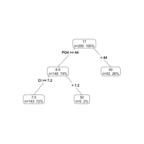
Illustration using a regression task
Forecasting Algae a1
library(DMwR); library(rpart.plot);
data(algae)
d <- algae[,1:12]
ar <- rpartXse(a1 ~ .,d, model=TRUE)
prp(ar,type=4,extra=101)
How to use the trees for Predicting?
tr <- d[1:150,]
ts <- d[151:200,]
ar <- rpartXse(a1 ~ .,tr, model=TRUE)
preds <- predict(ar,ts)
mae <- mean(abs(preds-ts$a1)); mae
## [1] 12.27911
cr <- cor(preds,ts$a1); cr
## [1] 0.512407
Hands-on Tree-based Models
Hands-on Tree-based Models
File Wine.data contains a data frame with data on green wine quality. The data set contains a series of tests with green wines (red and white). For each of these tests the values of several physicochemical variables together with a quality score assigned by wine experts (column Proline) is depicted.
Build a regression tree for the data set
Obtain a graph of the obtained regression tree
Apply the tree to the data used to obtain the model and calculate the mean squared error of the predictions
Split the data set in two parts: 70% of the tests (training data) and the remaining 30% (test data). Use the larger part to obtain a regression tree and apply it to the other part. Calculate the mean squared error again, and compare with the previous scores.
Naíve Bayes
Bayesian Classification
Naive Bayes
- Bayesian classifiers are statistical classifiers - they predict the probability that a case belongs to a certain class
- Bayesian classification is based on the Bayes’ Theorem (up next)
- A particular class of Bayesian classifiers - the Naïve Bayes Classifier - has shown rather competitive performance on several problems even when compared to more "sophisticated" methods
- Naïve Bayes is available in R on package
e1071, through functionnaiveBayes()
The Bayes’ Theorem - 1
- Let \(D\) be a data set formed by \(n\) cases \(\left \{ < \mathbf{x_i}, y_i > \right \}_{i=1}^N\), where \(\mathbf{x}\) is a vector of p variable values and \(y\) is the value on a target nominal variable \(Y\)
- Let \(H\) be a hypothesis that states that a certain test cases belongs to a class \(c \in Y\)
- Given a new test case \(\mathbf{x}\) the goal of classification is to estimate \(P(H | \mathbf{x})\), i.e. the probability that \(H\) holds given the evidence \(\mathbf{x}\)
- More specifically, we want to estimate the probability of each of the possible values given the test case (evidence) \(\mathbf{x}\)
The Bayes’ Theorem - 2
- \(P(H | \mathbf{x})\) is called the posterior probability, or a posteriori probability, of \(H\) conditioned on $\mathbf{x}
- We can also talk about \(P(H)\), the prior probability, or a priori probability, of the hypothesis \(H\)
- Notice that \(P(H | \mathbf{x})\) is based on more information than \(P(H)\), which is independent of the observation \(\mathbf{x}\)
- Finally, we can also talk about \(P(\mathbf{x} | H)\) as the posterior probability of \(\mathbf{x}\) conditioned on \(H\)
Bayes Theorem
$\large{P(H|\mathbf{x}) = \frac{P(\mathbf{x}|H) P(H)}{P(\mathbf{x})}}$
The Naive Bayes Classifier
How does it work?!
We have a data set \(D\) with cases belonging to one of m classes \(c_1, c_2, \cdots, c_m\)
Given a new test case \(\mathbf{x}\) this classifier produces as prediction the class that has the highest estimated probability, i.e. \(max_{i \in {1, 2, \cdots, m}} P(c_i|\mathbf{x})\)
Given that \(P(\mathbf{x})\) is constant for all classes, according to the Bayes Theorem the class with the highest probability is the one maximizing the quantity \(P(\mathbf{x}|c_i) P(c_i)\)
Naïve Bayes in R
library(e1071); sp <- sample(1:150, 100)
tr <- iris[sp, ]; ts <- iris[-sp, ]
nb <- naiveBayes(Species ~ ., tr)
(mtrx <- table(predict(nb, ts), ts$Species))
##
##              setosa versicolor virginica
##   setosa         14          0         0
##   versicolor      0         16         2
##   virginica       0          2        16
(err <- 1 - sum(diag(mtrx)) / sum(mtrx))
## [1] 0.08
head(predict(nb, ts, type='raw'), 2)
##      setosa   versicolor    virginica
## [1,]      1 1.115293e-17 3.730156e-28
## [2,]      1 1.209394e-13 5.587356e-23
Laplace Correction (important)
What if one of the components of the Bayes Theorem is equal to zero?
- This can easily happen in nominal variables if one of the values does not occur in a class, and would make the product equal to zero
- This zero probability would cancel the effects of all other probabilities
- The Laplace correction or Laplace estimator is a technique for probability estimation that tries to overcome these issues
- It consist in estimating \(P(\mathbf{x_k} | c_i)\) by \(\frac{|D_{x_k},c_i| + q}{|D_{c_i}| + q}\) , where \(q\) is an integer greater than zero (typically \(1\))
The Laplace Correction in R
library(e1071); sp <- sample(1:150,100)
tr <- iris[sp,]; ts <- iris[-sp,]
nb <- naiveBayes(Species ~ ., tr,laplace=1)
(mtrx <- table(predict(nb,ts),ts$Species))
##
##              setosa versicolor virginica
##   setosa         15          0         0
##   versicolor      0         18         1
##   virginica       0          3        13
(err <- 1-sum(diag(mtrx))/sum(mtrx))
## [1] 0.08
head(predict(nb,ts,type='raw'),2)
##      setosa   versicolor    virginica
## [1,]      1 1.636668e-18 2.342638e-28
## [2,]      1 3.748327e-19 1.061047e-28
Hands-on Bayesian Classifier
Hands-on Bayesian Classifier
Using the dataset iris, and remembering that the target variable is Species:
Separate the data set into 70% / 30% for training and test set, respectively
Build a Bayesian Classifier for the data set
Calculate the Accuracy metric
Rebuild the Bayesian Classifier with a Laplace Correction, and calculate the Accuracy metric once more.