

Predictive Modelling 2
Fraud Detection Course - 2020/2021
Nuno Moniz
nuno.moniz@fc.up.pt
Today
- k-Nearest Neighbors
- Support Vector Machines
k-Nearest Neighbors
k-Nearest Neighbors
- The k-nearest neighbor method was first described in the early 1950s.
- This method is computationally intensive with large data sets and it did not enjoy lots of popularity because of this.
- With the advent of cheap computing power its popularity has increased a lot because it is a very simple and effective method that can easily handle both classification and regression problems.
- k-nearest neighbors can be seen as methods that learn by analogy - i.e. they are based on the notion of similarity between cases.
k-Nearest Neighbors
The Basic Idea!
- If we are given a new test case x for which we want a prediction
- search in the training set for the most similar cases (the nearest neighbors) to x
- use the outcomes of these cases to obtain the prediction for x
kNN: Main Characteristics
- The k-nearest neighbors are known as lazy learners as they do not learn any model of the data
- Learning in k-nearest neighbors consists simply in storing the training data
- Variants here include storing in data structures that provide efficient querying of the nearest neighbors
- They do not make any assumption on the unknown functional form we are trying to approximate, which means that with sufficient data they are applicable to any problem
- They usually achieve good results but...
- They require a proper distance metric to be defined - issues like normalization, irrelevant variables, unknown values, etc., may have a strong impact on their performance
- They have fast training time, but slow prediction time
The Notion of Similarity
- The key issue on kNN is the notion of similarity
- This notion is strongly related with the notion of distance between observations
- Distances among observations in a data set can be used to find the neighbors of a test case
How to Calculate the Distance between 2 Cases?
- The notion of distance is related to the differences between the values on the variables describing the cases
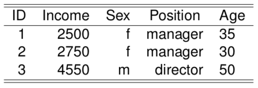
Case 1 is “closer” to case 2 than to 3
The Euclidean Distance Function
$\large{d(\mathbf{x,y}) = \sqrt{\sum_{i=1}^p (x_i - y_i)^2} }$
where \(x_i\) is the value of case x on variable i
Example!
- Given two cases \(\mathbf{x} = < 3, 5, 1 >\) and \(\mathbf{y} = < 12, 5.4, -3 >\) their Euclidean distance is given by:
$\large{d(\mathbf{x,y}) = \sqrt{\sum_{i=1}^p (x_i - y_i)^2} }$ $\large{d(\mathbf{x,y}) = \sqrt{(3-12)^2 + (5-5.4)^2 + (1-(-3))^2 } }$
A Generalization - the Minkowski distance
$d(\mathbf{x,y}) = \left ( \sum_{i=1}^p | x_i - y_i |^r \right )^{1/r}$
- where if
- r = 1 we have what is known as the Manhattan distance (or L1-norm)
- r = 2 we have the Euclidean distance
- etc.
Potential Problems with Distance Calculation
- In domains where cases are described by many variables several problems may arise that may distort the notion of distance between any two cases.
- Different scales of variables
- Different importance of variables
- Different types of data (e.g. both numeric and nominal variables, ...)
- etc.
Heterogeneous Distance Functions
How to calculate the distance between two cases described by variables with different type (e.g. numeric and nominal variables)? A possible solution,
$\large{ d(\mathbf{x,y}) = \left ( \sum_{i=1}^p \Delta_i (x_i, y_i) \right ) }$
where,
$\delta_i(x_i,y_i) = \left\{\begin{matrix} 1 & \text{if i is nominal and } v_1 \neq v_2 \\ 0 & \text{if i is nominal and } v_1 = v_2 \\ \frac{|v_1-v_2|}{range(i)} & \text{if i is numeric} \end{matrix}\right.$
The distance between \(<2500, f, director>\) and \(<2750, f, director>\) would be given by \(\frac{|2500-2750|}{range(Salary)} + 0 + 0 + \frac{|35-30|}{range(Age)}\)
1-Nearest Neighbor Classifier
Method
- Search for the training case most similar to the test case
- Predict for the test case the class of this nearest neighbor
Very simple method
May suffer with the presence of outliers
Frequently achieves good results
k-Nearest Neighbor Classifier
- Use the k nearest neighbors to obtain the classification of the test case
- Namely, the majority class on the k neighbors is the prediction of the mehtod
- What should be the value of k?
- Frequent values are 3, 5 and 7
- Odd numbers to avoid draws!
- It can be estimated experimentally
- Global estimation searches for the ideal k for a given data set
- Local estimation methods try to estimate the ideal k for each test case (computationally very demanding!)
k-nearest neighbors in R
- Package class contains function
knn()
library(class)
sp <- sample(1:150,100)
tr <- iris[sp,]; ts <- iris[-sp,]
nn3 <- knn(tr[,-5],ts[,-5],tr[,5],k=3)
(mtrx <- table(nn3,ts$Species))
##
## nn3          setosa versicolor virginica
##   setosa         10          0         0
##   versicolor      0         19         1
##   virginica       0          2        18
(err <- 1-sum(diag(mtrx))/sum(mtrx))
## [1] 0.06
k-nearest neighbors in R - 2
- Package DMwR has a wrapper function with a "standard"" interface,
library(class); library(DMwR)
## Loading required package: lattice
## Loading required package: grid
## Registered S3 method overwritten by 'quantmod':
##   method            from
##   as.zoo.data.frame zoo
sp <- sample(1:150,100)
tr <- iris[sp,]; ts <- iris[-sp,]
nn3 <- kNN(Species ~ .,tr,ts,k=3,norm=TRUE)
(mtrx <- table(nn3,ts$Species))
##
## nn3          setosa versicolor virginica
##   setosa         18          0         0
##   versicolor      0         12         2
##   virginica       0          2        16
(err <- 1-sum(diag(mtrx))/sum(mtrx))
## [1] 0.08
Trying to find the "ideal" value of k in R
trials <- c(1,3,5,7,11); nreps <- 10
res <- matrix(NA, nrow=length(trials), ncol=2)
for(k in seq_along(trials)) {
  errs <- rep(0,nreps)
  for(r in 1:nreps) {
    sp <- sample(1:150,100); tr <- iris[sp,]; ts <- iris[-sp,]
    nn3 <- kNN(Species ~ .,tr,ts,k=trials[k],norm=TRUE)
    mtrx <- table(nn3,ts$Species)
    errs[r] <- 1-sum(diag(mtrx))/sum(mtrx)
  }
  res[k,] <- c(mean(errs),sd(errs))
}
dimnames(res) <- list(paste('k',trials,sep='='),c('avg','std'))
res
##        avg        std
## k=1  0.074 0.04115013
## k=3  0.054 0.03777124
## k=5  0.046 0.02988868
## k=7  0.044 0.02458545
## k=11 0.056 0.03373096
k-Nearest Neighbor Regression
- Method
- Search for the training case most similar to the test case
- Predict for the test case the average of the target variable values of the neighbors
k-Nearest Neighbors regression in R
- Package caret has a function that to obtain these models
library(caret)
data(Boston,package="MASS")
sp <- sample(1:506,354)
tr <- Boston[sp,]
ts <- Boston[-sp,]
tgt <- which(colnames(Boston) == "medv")
nn3 <- knnreg(tr[,-tgt],tr[,tgt],k=3)
pnn3 <- predict(nn3,ts[,-tgt])
(mse <- mean((pnn3-ts[,tgt])^2))
## [1] 46.14592
Hands-on kNN
Hands-on kNN
- Using the iris data set that comes with R answer the following questions:
Build a distance matrix between all cases (lookup the function
dist())Load the data and split it in two random partitions: one with 100 cases that will form the training set; and the other with the remaining 50 that are the test cases.
Using the previously obtained distance matrix: how would you find the 2 nearest neighbours of the first test case?
Using the strategy of the previous question what would be the prediction for the same test case if we used 3, 5 or 7 nearest neighbours?
Obtain the predictions for all test cases using the 3 nearest neighbours strategy (without using the function knn())
Obtain the confusion matrix and the error rate of the previous predictions
Support Vector Machines
SVM's! A Bit of History...
- SVM’s were introduced in 1992 at the COLT-92 conference
- They gave origin to a new class of algorithms named kernel machines
- Since then there has been a growing interest on these methods
- More information may be obtained at www.kernel-machines.org
- A good reference on SVMs:
- N. Cristianini and J. Shawe-Taylor: An introduction to Support Vector Machines. Cambridge University Press, 2000.
- SVMs have been applied with success in a wide range of areas like: bio-informatics, text mining, hand-written character recognition, etc.
Two Linearly Separable Classes
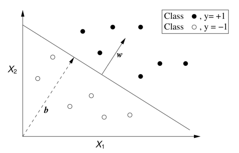
- Obtain a linear separation of the cases (binary classification problems)
- Very simple and effective for linearly separable problems
- Most real-world problems are not linearly separable!
The Basic Idea of SVMs
- Map the original data into a new space of variables with very high dimension.
- Use a linear approximation on this new input space.
The Idea in a Figure
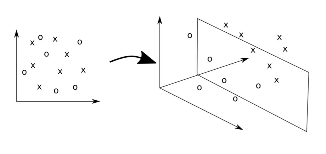
Map the original data into a new (higher dimension) coordinates system where the classes are linearly separable
Maximum Margin Hyperplane
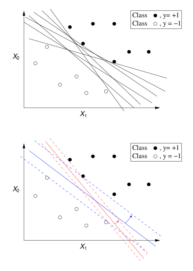
- There is an infinite number of hyperplanes separating the two classes!
- Which one should we choose?!
- We want the one that ensures a better classification accuracy on unseen data
- SVMs approach this problem by searching for the maximum margin hyperplane
The Support Vectors
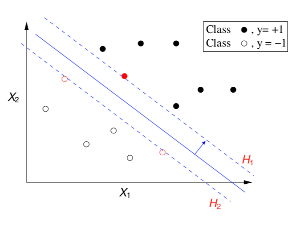
- All cases that fall on the hyperplanes H1 and H2 are called the support vectors.
- Removing all other cases would not change the solution!
The Optimal Hyperplane
- SVMs use quadratic optimization algorithms to find the optimal hyperplane that maximizes the margin that separates the cases from the 2 classes
- Namely, these methods are used to find a solution to the following equation,
$L_D = \sum_{i=1}^n \alpha_i - \frac{1}{2} \sum_{i,j}^n \alpha_i \alpha_j y_i y_j (\mathbf{x_i} \cdot \mathbf{x_j})$
Subject to:
\(\alpha_i \geq 0\) \(\sum_i \alpha_i y_i = 0\)
In the found solution, the \(\alpha_i\)'s \(> 0\) correspond to the support vectors that represent the optimal solution
Recap
- Most real world problems are not linearly separable
- SVMs solve this by "moving" into a extended input space where classes are already linearly separable
- This means the maximum margin hyperplane needs to be found on this new very high dimension space
The Kernel trick
- The solution to the optimization equation involves dot products that are computationally heavy on high-dimensional spaces
- It was demonstrated that the result of these complex calculations is equivalent to the result of applying certain functions (the kernel functions) in the space of the original variables.
The Kernel Trick
Instead of calculating the dot products in a high dimensional space, take advantage of the proof that \(K(\mathbf{x,z}) = \phi(\mathbf{x}) \cdot \phi(\mathbf{z})\) and simply replace the complex dot products by these simpler and efficient calculations
Summary of the SVMs Method
- As problems are usually non-linear on the original feature space, move into a high-dimension space where linear separability is possible
- Find the optimal separating hyperplane on this new space using quadratic optimization algorithms
- Avoid the heavy computational costs of the dot products using the kernel trick
How to handle more than 2 classes?
- Solve several binary classification tasks
- Essentially find the support vectors that separate each class from all others
The Algorithm
- Given a m classes task
- Obtain m SVM classifiers, one for each class
- Given a test case assign it to the class whose separating hyperplane is more distant from the test case
Obtaining an SVM in R
The package e1071
library(e1071)
data(Glass,package='mlbench')
tr <- Glass[1:200,]
ts <- Glass[201:214,]
s <- svm(Type ~ .,tr)
predict(s,ts)
## 201 202 203 204 205 206 207 208 209 210 211 212 213 214
##   7   2   7   7   7   7   7   2   7   7   7   7   7   7
## Levels: 1 2 3 5 6 7
Obtaining an SVM in R (cont.)
The package e1071
ps <- predict(s,ts)
table(ps,ts$Type)
##
## ps   1  2  3  5  6  7
##   1  0  0  0  0  0  0
##   2  0  0  0  0  0  2
##   3  0  0  0  0  0  0
##   5  0  0  0  0  0  0
##   6  0  0  0  0  0  0
##   7  0  0  0  0  0 12
mc <- table(ps,ts$Type)
error <- 100*(1-sum(diag(mc))/sum(mc))
error
## [1] 14.28571
\(\epsilon\)-SV Regression
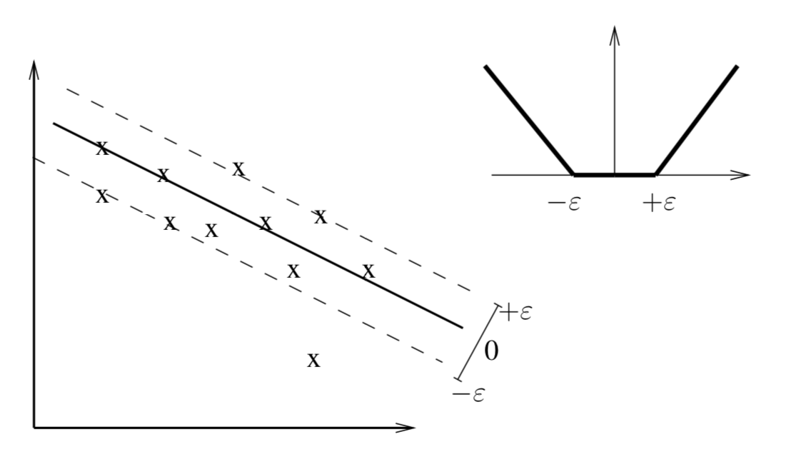
- Vapnik (1995) proposed the notion of \(\epsilon\) support vector regression
- The goal in \(\epsilon\)-SV Regression is to find a function \(f(x)\) that has at most \(\epsilon\) deviation from the given training cases
- In other words we do not care about errors smaller than \(\epsilon\)
V. Vapnik (1995). The Nature of Statistical Learning Theory. Springer.
\(\epsilon\)-SV Regression (cont.)
- \(\epsilon\)-SV Regression uses the following error metric,
$| \xi |_\epsilon = \left\{\begin{matrix} 0 & | \xi | \leq \epsilon \\ | \xi | - \epsilon & \text{otherwise} \end{matrix}\right.$
\(\epsilon\)-SV Regression (cont.)
- The theoretical development of this idea leads to the following optimization problem,
Minimize: \(\large{\frac{1}{2} || \mathbf{w} ||^2 + C \sum_{i=1}^I (\xi_i + \xi_i^\star )}\)
Subject to:
$\left\{\begin{matrix} y_i - \mathbf{w} \cdot \mathbf{x} - b & \leq \epsilon + \xi_i \\ \mathbf{w} \cdot \mathbf{x} + b - y_i & \leq \epsilon + \xi_i^{\star} \\ \xi_i, \xi_i^{\star} & \geq 0 \end{matrix}\right.$
where \(C\) corresponds to the cost to pay for each violation of the error limit \(\epsilon\)
\(\epsilon\)-SV Regression (cont.)
- As within classification we use the kernel trick to map a non-linear problem into a high dimensional space where we solve the same quadratic optimization problem as in the linear case
- In summary, by the use of the \(|\xi|_{\epsilon}\) loss function we reach a very similar optimization problem to find the support vectors of any non-linear regression problem.
SVMs for regression in R
library(e1071)
library(DMwR)
data(Boston,package='MASS')
sp <- sample(1:nrow(Boston),354)
tr <- Boston[sp,]
ts <- Boston[-sp,]
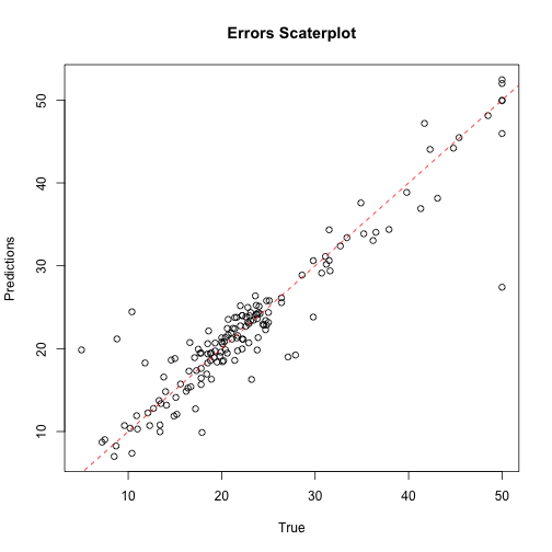
s <- svm(medv ~ .,tr,cost=10,epsilon=0.02)
preds <- predict(s,ts)
regr.eval(ts$medv,preds)
##        mae        mse       rmse       mape
##  2.0674690 12.5715754  3.5456417  0.1214812
plot(ts$medv,preds,main='Errors Scaterplot',
     ylab='Predictions',xlab='True')
abline(0,1,col='red',lty=2)
Hands-on SVMs
File Wine.data contains a data frame with data on green wine quality. The data set contains a series of tests with green wines (red and white). For each of these tests the values of several physicochemical variables together with a quality score assigned by wine experts (column Proline) is depicted.
Obtain an SVM model for forecasting the quality of variant with Class 2
Split the data set in two parts: one with 70% of the samples and the other with the remaining 30%. Obtain an SVM with the first part and apply it to the second. What was the resulting mean absolute error?
Using the
round()function, round the predictions obtained in the previous question to the nearest integer. Calculate the error rate of the resulting integers when compared to the true values
