

Predictive Modelling 3
Fraud Detection Course - 2020/2021
Nuno Moniz
nuno.moniz@fc.up.pt
Today
- Ensembles
- Clustering
Ensembles
Ensemble Models
What?
- Ensembles are collections of models that are used together to address a certain prediction problem
Why? (Diettrich, 2002)
- For complex problems it is hard to find a model that "explains" all observed data
- Averaging over a set of models typically leads to significantly better results
Dietterich, T. G. (2002). Ensemble Learning. In The Handbook of Brain Theory and Neural Networks, Second edition, (M.A. Arbib, Ed.), pp. 405-408. The MIT Press.
Bias-Variance Trade-off
The Bias-Variance Decomposition of Prediction Error
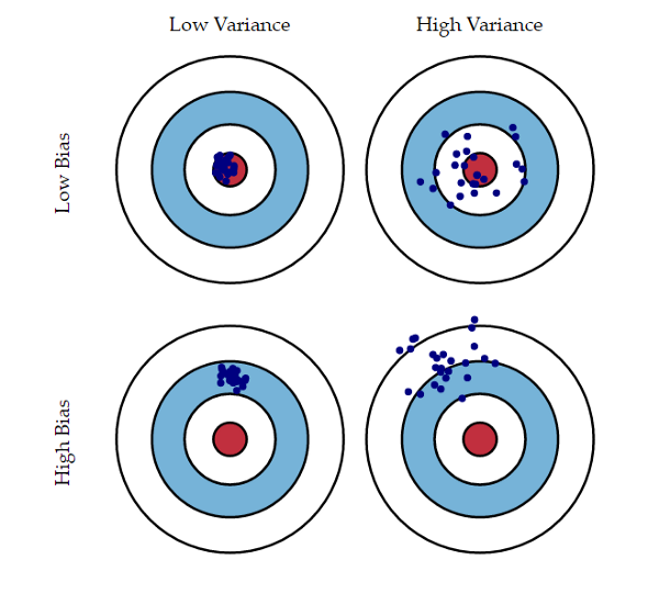
- The prediction error of a model can be split in two main components: the bias and the variance components
- The bias component is the part of the error that is due to the poor ability of the model to fit the seen data
- The variance component has to do with the sensibility of the model to the given training data
Bias-Variance Trade-off
- Decreasing the bias by adjusting more to the training sample will most probably lead to a higher variance - the over-fitting phenomenon
- Decreasing the variance by being less sensitive to the given training data will most probably have as consequence a higher bias
Result: there is a well-known bias-variance trade-off in learning a prediction model
Ensembles? They are able to reduce both components of the error
Their approach consists on applying the same algorithm to different samples of the data and use the resulting models in a voting/averaging schema to obtain predictions for new cases
Bias-Variance Trade-off
Expected error
$E \left [ \left ( y - \hat{f} \left ( x \right ) \right )^2 \right ] = \left ( {Bias} \left [ \hat{f} \left ( x \right ) \right ] \right )^2 + {Var} \left [ \hat{f} \left ( x \right ) \right ] + \sigma^2$
Bias
${Bias} \left [ \hat{f} \left ( x \right ) \right ] = E \left [ \hat{f} \left ( x \right ) \right ] - f \left ( x \right )$
Variance
${Var} \left [ \hat{f} \left ( x \right ) \right ] = E \left [ \hat{f} \left ( x \right )^2 \right ] - E \left [ \hat{f} \left ( x \right ) \right ]^2$
Bias-Variance Trade-off (Translated)
The expected error of a certain model m on an unseen case is equal to the sum of its
- squared bias
- variance, and
- irreducible error
Bias: the distance between the average value of predictions and the true value of the unseen case
Variance: the distance between the average of the squared predicted values and the average of the predicted values squared
Irreducible error: The previous components are all positive - this component sets the lower bound on the expected error
Bias-Variance Trade-off (illustration)
Under and overfitting (illustration)

Under and overfitting (attempt at humour)


Types of approaches
Independent or Parallel Models
- One of the ways of obtaining an ensemble is to construct them independently in a way that ensures some diversity among them
*There are several ways we can reach this diversity among which we may refer:
- Applying the models on somewhat different training sets
- Applying the models on data sets using different predictors
Coordinated (or Sequential) Models
- Another way of obtaining an ensemble is to construct a "larger" model by composing it from smaller models integrated somehow where each simpler model has some weighted participation in the ensemble predictions
- The task of this type of ensembles is then to choose the right component models and their respective weight, so that the weighted sum of these components has a good predictive performance
Bagging
- Bagging (Breiman, 1996) or Bootstrap Aggregating is a method that obtains a set of k models using different bootstrap samples of the given training data
- For each model a sample with replacement of the same size as the available data is obtained
- This means that for each model there is a small proportion of the examples that will be different
- If the base learner has a high variance (i.e. very sensitive to variations on the training sample), this will ensure diversity among the k models
- In this context, bagging should be applied to base learners with high variance
Breiman, L. (1996): Bagging predictors. In Machine Learning, 24: 123–140.
A Simple Implementation of Bagging in R
simpleBagging <- function(form,data,model='rpartXse',nModels=100,...) {
  ms <- list()
  n <- nrow(data)

  for(i in 1:nModels) {
    tr <- sample(n,n,replace=T)
    ms[[i]] <- do.call(model,c(list(form,data[tr,]),...))
  }
  ms
}

predict.simpleBagging <- function(models,test) {
  ps <- sapply(models, function(m) predict(m,test))
  apply(ps,1,mean)
}
How to use it
data(Boston, package='MASS')
library(DMwR)

trPerc <- 0.7
sp <- sample(1:nrow(Boston), trPerc * nrow(Boston))
tr <- Boston[sp, ]
ts <- Boston[-sp, ]

m <- simpleBagging(medv ~ ., tr, nModels=300, se=0.5)
ps <- predict.simpleBagging(m, ts)
mean(abs(ps - ts$medv))
## [1] 2.203965
Package adabag
library(adabag)
data(iris)
trPerc <- 0.7
sp <- sample(1:nrow(iris), trPerc * nrow(iris))
tr <- iris[sp, ]; ts <- iris[-sp, ]
m <- bagging(Species ~ ., tr, mfinal = 50)
ps <- predict(m, ts)
ps$confusion
##                Observed Class
## Predicted Class setosa versicolor virginica
##      setosa          9          0         0
##      versicolor      0         12         0
##      virginica       0          5        19
ps$error
## [1] 0.1111111
Varying the Predictors
- Another way of generating a diverse set of models is by using different randomly chosen predictors
- The idea is similar to bagging but instead of generating samples of the cases we generate samples of the variables
Random Forests
- Random Forests (Breiman, 2001) put the ideas of sampling the cases and sampling the predictors, together in a single method
- Random Forests combine the ideas of bagging together with the idea of random selection of predictors
- Random Forests consist of sets of tree-based models where each tree is obtained from a bootstrap sample of the original data and uses some form of random selection of variables during tree growth
Breiman, L. (2001): "Random Forests". Machine Learning 45 (1): 5—32.
Random Forests - the algorithm
- For each of the k models
- Draw a random sample with replacement to obtain the training set
- Grow a classification or regression tree
- On each node of the tree choose the best split from a randomly selected subset m of the predictors
- The trees are fully grown, i.e. no pruning is carried out
Random Forests in R
The package randomForest (look into the ranger package also - faster)
library(randomForest)
data(Boston,package="MASS")
samp <- sample(1:nrow(Boston),354)
tr <- Boston[samp,]
ts <- Boston[-samp,]
m <- randomForest(medv ~ ., tr)
ps <- predict(m,ts)
mean(abs(ts$medv-ps))
## [1] 2.467972
A classification example
data(Glass,package='mlbench')
sp <- sample(1:nrow(Glass),150)
tr <- Glass[sp,]; ts <- Glass[-sp,]
m <- randomForest(Type ~ ., tr, ntree=200)
ps <- predict(m,ts)
table(ps,ts$Type)
##
## ps   1  2  3  5  6  7
##   1 17  3  5  0  0  1
##   2  1 19  0  0  0  2
##   3  0  0  1  0  0  0
##   5  0  1  0  3  0  0
##   6  0  0  0  0  2  0
##   7  0  0  0  0  0  9
A classification example (cont.)
mc <- table(ps,ts$Type)
err <- 100*(1-sum(diag(mc))/sum(mc))
err
## [1] 20.3125
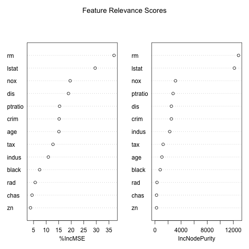
Other Uses of Random Forests: Variable Importance
data(Boston,package='MASS')
library(randomForest)
m <- randomForest(medv ~ ., Boston,
                  importance=T)
importance(m)
##           %IncMSE IncNodePurity
## crim    15.192643     2507.2427
## zn       3.776905      234.2308
## indus   10.882079     2260.5562
## chas     4.392328      242.1772
## nox     19.566910     3136.5959
## rm      37.051416    12803.6063
## age     15.099170     1060.0131
## dis     18.906455     2508.2821
## rad      5.649464      305.0809
## tax     12.739131     1247.6428
## ptratio 15.368937     2772.9928
## black    7.408346      796.7219
## lstat   29.521515    12158.9617
varImpPlot(m, main="Feature Relevance Scores")
Boosting
Boosting (Schapire, 1990) was developed with the goal of answering the question: Can a set of weak learners create a single strong learner?
- In the above question a "weak" learner is a model that alone is unable to correctly approximate the unknown predictive function, while a “strong” learner has that ability
- Boosting algorithms work by iteratively creating a strong learner by adding at each iteration a new weak learner to make the ensemble
- Weak learners are added with weights that reflect the learner’s accuracy
- After each addition the data is re-weighted such that cases that are still poorly predicted gain more weight
- This means that each new weak learner will focus on the errors of the previous ones
Rob Schapire (1990). Strength of Weak Learnability. Machine Learning Vol. 5, pages 197–227.
The AdaBoost Algorithm
- AdaBoost or Adaptive Boosting (Freund & Shapire, 1996) is an ensemble algorithm that can be used to improve the performance of a base algorithm
- It consists of an iterative process where new models are added to form an ensemble
- It is adaptive in the sense that at each new iteration of the algorithm the new models are built to try to overcome the errors made in the previous iterations
- At each iteration the weights of the training cases are adjusted so that cases that were wrongly predicted get their weight increased to make new models focus on accurately predicting them
- AdaBoost was created for classification although variants for regression exist
Y. Freund and R. Schapire (1996). Experiments with a new boosting algorithm, in Proc. of 13th International Conference on Machine Learning
AdaBoost for Classification in R
Package adabag
library(adabag)
data(iris)

trPerc <- 0.7
sp <- sample(1:nrow(iris),as.integer(trPerc*nrow(iris)))
tr <- iris[sp,]
ts <- iris[-sp,]

m <- boosting(Species ~ ., tr)
ps <- predict(m,ts)
ps$confusion
##                Observed Class
## Predicted Class setosa versicolor virginica
##      setosa         12          0         0
##      versicolor      0         16         0
##      virginica       0          2        15
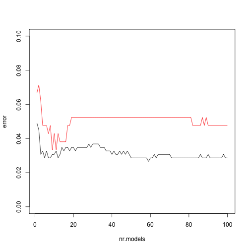
Error curves
This package also includes a function that allows you to check the evolution of the error as you increase the number of weak learners.
library(adabag)
data(BreastCancer,package="mlbench")

trPerc <- 0.7
sp <- sample(1:nrow(BreastCancer),as.integer(trPerc*nrow(BreastCancer)))
tr <- BreastCancer[sp,-1]
ts <- BreastCancer[-sp,-1]
m <- bagging(Class ~ ., tr,mfinal=100)
ps <- predict(m,ts)
ptr <- errorevol(m,tr)
pts <- errorevol(m,ts)
Error curves (cont.)
plot(ptr$error,type="l",xlab="nr.models",ylab="error",ylim=c(0,0.1))
lines(pts$error,col="red")
AdaBoost for Regression in R
Package gbm
Package gbm implements the Gradient Boosting Machine (Friedman, 2001)
library(gbm)
## Loaded gbm 2.1.8
data(Boston,package='MASS')
trPerc <- 0.7
sp <- sample(1:nrow(Boston),as.integer(trPerc*nrow(Boston)))
tr <- Boston[sp,]; ts <- Boston[-sp,]
m <- gbm(medv ~ .,distribution='gaussian',data=tr, n.trees=20000,verbose=F)
ps <- predict(m,ts,type='response',n.trees=20000)
mean(abs(ps-ts$medv))
## [1] 3.198266
Hands-on Ensembles
Load in the data set algae and answer the following questions:
How would you obtain a random forest to forecast the value of alga
a4Repeat the previous exercise but now using a boosting model
Obtain the predictions of the two previous models for the data used to obtain them (the train set). Draw a scatterplot comparing these predictions
Load the data set
testAlgae. It contains a data frame namedtest.algaewith some extra 140 water samples for which we want predictions. Use the previous two models to obtain predictions for a4 on these new samples. Check what happened to the test cases with NA’s. Fill-in the NA’s on the test set (remember the functionknnImputation()from theDMwRpackage) and repeat the experiment.
Clustering
Clustering
Descriptive Analytics
Generic Goals of Descriptive Analytics
- Predictive Analytics has to do with forecasting
- Descriptive Analytics has to do with describing/summarizing or finding structure on what we have observed
- Data summarization and visualization can be seen as simple forms of descriptive analytics
- However, most frequently descriptive modeling is associated with clustering
Clustering
Generic Goals of Clustering
- Obtain the "natural" grouping of a set of data - i.e. find some structure on the data set
- Observations on the same group are supposed to share some properties, i.e. being similar
- Provide some abstraction of the found groups (e.g. a representation of their main features; a prototype for each group; etc.)
The Notion of Similarity
- The key issue on clustering is the notion of similarity
- This notion is strongly related with the notion of distance between observations
- Most methods use the information on the distances among observations in a data set to decide on the natural groupings of the cases
Remember the Euclidean, Minkoswki and heterogeneous distance functions from the previous class?
Distance functions in R
Function dist() can be used to obtain a distance matrix between a set of cases
data(iris)
dm <- dist(iris[,-5]) # excluding the nominal target
as.matrix(dm)[1,4] # because dm is of class "dist"
## [1] 0.6480741
Parameter method of function dist() allows you to specify different types of functions (defaults to Euclidean), such as Manhattan or Minkowski (check the help of the function)
Note that this function only accepts numeric variables
Mixed Type Distance functions in R
Function daisy() from package cluster can calculate distances between cases that include both numeric and nominal variables (heterogeneous distance)
library(cluster)
data(iris)
dm <- daisy(iris)
as.matrix(dm)[1,4] # because dm is of class "dist"
## [1] 0.06450094
Parameter metric of function daisy() allows you to specify different types of functions (defaults to Euclidean), namely Euclidean, Manhattan or Gower (check the help of the function)
Main Types of Clustering Methods
Hierarchical or Partitional
- Hierarchical
- Generate a hierarchy of groups, from 1 to n groups, where n is the number of lines in the data set
- Agglomerative: generate a hierarchy from bottom to top (from n to 1 group)
- Divisive: create a hierarchy in a top down way (from 1 to n groups)
- Generate a hierarchy of groups, from 1 to n groups, where n is the number of lines in the data set
- Partitional
- Divide the observations in k groups according to some criterion
Main Types of Clustering Methods (cont.)
Exclusive or with Overlapping
- Exclusive
- Each observation is assigned to a single group
- With overlapping
- Each observation may belong to more that one group with different degrees of membership
Partitional Methods
Introduction
Goal: Partition the given set of data into \(k\) groups by either minimizing or maximizing a pre-specified criterion
Some key issues:
- The user needs to select the number of groups
- The number of possible divisions of \(n\) cases into \(k\) groups can grow fast!
$N(n,k) = \frac{1}{k!} \sum_{i=1}^k (-1)^{k-i} \binom{k}{i} i^n$
e.g. for \(n = 100\) and \(k = 5\), \(N(100, 5) \approx 6.6 \cdot 10^{67}\)
Partitional Methods
Partitioning Criteria
- (Some) Cluster properties
- Cluster compactness - how similar are cases within the same cluster
- Cluster separation - how far is the cluster from the other clusters
- (Some) Criteria for numeric data
- Sum of squares - \(h(c) = \sum_{x \in c} \sum_{i=1}^a (v_{x,i} - \bar{v}_i^c)^2\)
- \(L_1\) measure - \(h(c) = \sum_{x \in c} \sum_{i=1}^a | v_{x,i} - \tilde{v}_i^c |\)
\(\bar{v}_i^c\) is the average value of variable \(i\) in cluster \(c\), and \(\tilde{v}_i^c\) the median
Partitional Methods
The k-Means Method
It is a very simple partition-based method that obtains \(k\) groups of a data set
The algorithm
- Initialize the centers of the k groups to a set of randomly chosen observations
- Repeat
- Allocate each observation to the group whose center is nearest
- Re-calculate the center of each group
- Until the groups are stable
Partitional Methods
Observations on the k-Means Method
- It uses the squared Euclidean distance as criterion
- Maximizes inter-cluster dissimilarity
- It does not ensure an optimal clustering
- We may obtain different solutions with different starting points
Partitional Methods
k-Means in R
data(iris)
k3 <- kmeans(iris[,-5],centers=3,iter.max=200)
k3
## K-means clustering with 3 clusters of sizes 38, 50, 62
##
## Cluster means:
##   Sepal.Length Sepal.Width Petal.Length Petal.Width
## 1     6.850000    3.073684     5.742105    2.071053
## 2     5.006000    3.428000     1.462000    0.246000
## 3     5.901613    2.748387     4.393548    1.433871
##
## Clustering vector:
##   [1] 2 2 2 2 2 2 2 2 2 2 2 2 2 2 2 2 2 2 2 2 2 2 2 2 2 2 2 2 2 2 2 2 2 2 2 2 2
##  [38] 2 2 2 2 2 2 2 2 2 2 2 2 2 3 3 1 3 3 3 3 3 3 3 3 3 3 3 3 3 3 3 3 3 3 3 3 3
##  [75] 3 3 3 1 3 3 3 3 3 3 3 3 3 3 3 3 3 3 3 3 3 3 3 3 3 3 1 3 1 1 1 1 3 1 1 1 1
## [112] 1 1 3 3 1 1 1 1 3 1 3 1 3 1 1 3 3 1 1 1 1 1 3 1 1 1 1 3 1 1 1 3 1 1 1 3 1
## [149] 1 3
##
## Within cluster sum of squares by cluster:
## [1] 23.87947 15.15100 39.82097
##  (between_SS / total_SS =  88.4 %)
##
## Available components:
##
## [1] "cluster"      "centers"      "totss"        "withinss"     "tot.withinss"
## [6] "betweenss"    "size"         "iter"         "ifault"
Clustering Validation
How to validate/evaluate/compare the results obtained with some clustering method?
Related Questions
- Is the found group structure random?
- What is the "correct" number of groups?
- How to evaluate the result of a clustering algorithm when we do not have information on the number of groups in the data set?
- How to compare the results obtained by different methods when outside information on the number of groups exists?
- How to compare alternative solutions (e.g. obtained using different clustering algorithms)?
Types of Evaluation Measures
- Unsupervised - try to measure the quality of the clustering without any information on the "ideal" structure of the data
- Cohesion coefficients - determine how compacts/cohesive are the members of a group
- Separation coefficients - determine how different are the members of different groups
- Supervised - compare the obtained clustering (grouping) with the external information that we have available
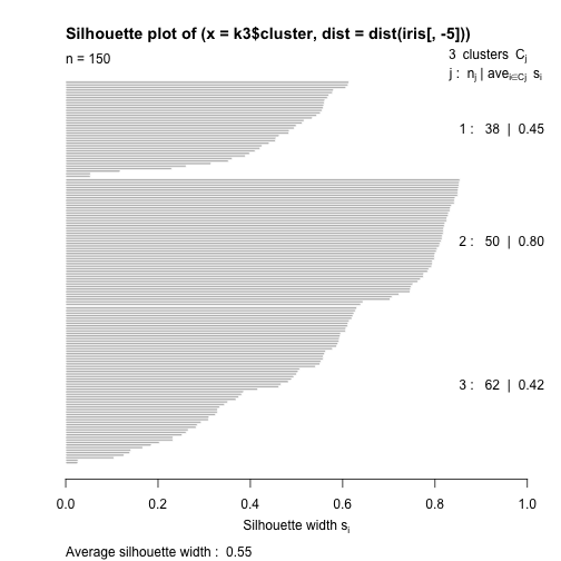
The Silhouette Coefficient (unsupervised measure)
Popular coefficient that tries to incorporate both the notions of cohesion and separation
- For each object \(i\) obtain the average distance to all objects in the same group and call this average \(a_i\)
- For each object \(i\) and any other group to which \(i\) does not belong, obtain the average distance to the members of these other groups. Obtain the minimum value of these distances and call it \(b_i\)
- The silhouette coefficient, s_i is equal to
$s_i = \frac{b_i - a_i}{max(a_i,b_i)}$
The coefficient takes values between \(-1\) and \(1\). Ideally all objects should have positive values (\(a_i < b_i\)), and the \(a_i\)'s should be near zero
An illustrative example with R
table(k3$cluster, iris$Species)
##
##     setosa versicolor virginica
##   1      0          2        36
##   2     50          0         0
##   3      0         48        14
library(cluster)
s <- silhouette(k3$cluster,
                dist(iris[, -5]))
plot(s)
How to Define the Number of Groups
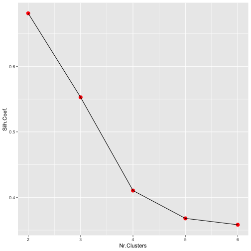
Among many different possible strategies we could use the average silhouette coefficient value to try several possible clusters and select the "best" one. An illustrative example in R:
d <- dist(iris[,-5])
avgS <- c()
for(k in 2:6) {
  cl <- kmeans(iris[,-5],centers=k,iter.max=200)
  s <- silhouette(cl$cluster,d)
  avgS <- c(avgS,mean(s[,3]))
}
library(ggplot2)
ggplot(data.frame(nClus=2:6,Silh=avgS),
       aes(x=nClus,y=Silh)) +
  geom_point(size=3,color="red") +
  geom_line() + xlab("Nr.Clusters") +
  ylab("Silh.Coef.")
The Partition Around Medoids Method
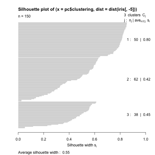
- The PAM algorithm searches for the \(k\) representative objects (the medoids) among the cases in the given data set.
- As with k-means each observation is allocated to the nearest medoid.
- PAM is more robust to the presence of outliers because it uses original objects as centroids instead of averages that may be subject to the effects of outliers.
- Moreover PAM uses a more robust measure of the clustering quality, an absolute error instead of the squared error used in k-means,
$H(C,k) = \sum_{i=1}^k \sum_{\mathbf{x} \in C_i} | \mathbf{x} - \bar{\mathbf{x}}_{C_i} |$
where \(\bar{\mathbf{x}}_{C_i}\) is the centroid of cluster \(C_i\)
An example with R
library(cluster)
pc <- pam(iris[,-5],k=3)
table(pc$clustering,iris$Species)
##
##     setosa versicolor virginica
##   1     50          0         0
##   2      0         48        14
##   3      0          2        36
s <- silhouette(pc$clustering,
                dist(iris[,-5]))
plot(s)
The CLARA Clustering Method
- The PAM algorithm has several advantages in terms of robustness when compared to k-means.
- However, these advantages come at the price of additional computational complexity that may be too much for very large data sets
- CLARA tries to solve these efficiency problems
- It does that by using sampling, i.e. working on parts of the data set instead of the full data set (think PA1)
The CLARA Algorithm
- Repeat n times the following:
- Draw a random sample of size m
- Apply PAM to this random sample to obtain k centroids
- Allocate the full set of observations to one of these centroids
- Calculate sum of dissimilarities of the resulting clustering (as in PAM)
- Return as result the clustering of the n repetitions that got lowest sum of dissimilarities
An example with R
library(cluster)
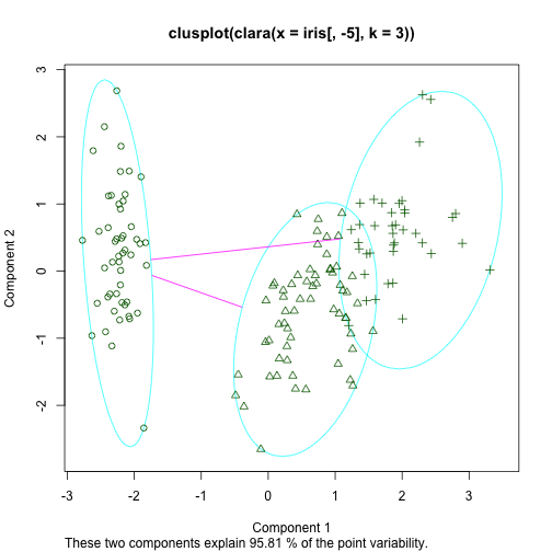
cl <- clara(iris[,-5],3)
table(cl$clustering,iris$Species)
##
##     setosa versicolor virginica
##   1     50          0         0
##   2      0         48        13
##   3      0          2        37
clusplot(cl)
clusplot(cl)
The DBSCAN Method
- This is a partition based method based on the notion of "density" of the observations
- Key Idea: The density of a single observation is estimated by the number of observations that are within a certain radius (a parameter of the method)
- Based on this idea observations are classified as:
- core points: if the number of observations within its radius are above a certain threshold
- border points: if the number of observations within their radius does not reach the threshold but they are within the radius of a core point
- noise points: they do not have enough observations within their radius, nor are they sufficiently close to any core point
The DBSCAN Method (cont.)
The DBSCAN Algorithm
- Classify each observation in one of the three possible alternatives
- Eliminate the noise points from the formation of the groups
- All core points that are within a certain distance of each other are allocated to the same group
- Each border point is allocated to the group of the nearest core point
Note that this method does not require the user to specify the number of groups.
(But, you need to specify the radius)
Applying DBSCAN to Iris
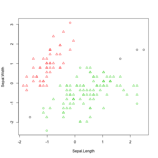
library(fpc)
d <- scale(iris[,-5])
db <- dbscan(d,0.9)
db
## dbscan Pts=150 MinPts=5 eps=0.9
##        0  1  2
## border 4  1  4
## seed   0 48 93
## total  4 49 97
table(db$cluster,iris$Species)
##
##     setosa versicolor virginica
##   0      1          0         3
##   1     49          0         0
##   2      0         50        47
plot(db, d)
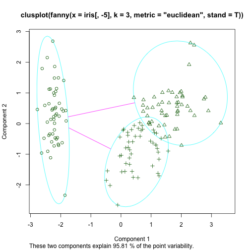
Fuzzy Clustering using FANNY
- FANNY is a partition based method that has the particularity of producing cluster membership scores for each observation.
- This means that each observation has \(k\) membership scores (summing up to 1)
Applying FANNY to Iris
library(cluster)
f <- fanny(iris[,-5], 3, stand=T,metric='euclidean')
head(f$membership)
##           [,1]       [,2]      [,3]
## [1,] 0.8297737 0.07841458 0.0918117
## [2,] 0.6409940 0.15528310 0.2037229
## [3,] 0.7534768 0.10943177 0.1370914
## [4,] 0.6870170 0.13724986 0.1757331
## [5,] 0.7931229 0.09626758 0.1106095
## [6,] 0.6080978 0.18974175 0.2021604
table(f$clustering,iris$Species)
##
##     setosa versicolor virginica
##   1     50          0         0
##   2      0         12        39
##   3      0         38        11
clusplot(f)
Hierarchical Clustering
- Goal: Obtain a hierarchy of groups, where each level represents a possible solution with x groups. It is up to the user to select the solution he wants.
- Agglomerative Methods
- Start with as many groups as there are cases
- On each upper level a pair of groups is merged into a single group
- The chosen pair is formed by the groups that are more similar
- Divisive Methods (much less used)
- Start with a single group
- On each level select a group to be split in two
- The selected group is the one with smallest uniformity
Agglomerative Hierarchical Clustering
The difference among two groups, candidates for merging can be measure in several ways:
- The single linkage method
- The difference among two groups is measured by the smallest distance between any two observations in each group
- The complete linkage method
- The difference between two groups is measured by the largest distance between any two observations of the groups
- The average linkage method
- The difference between two groups is measured by the average distance between any two observations of the groups
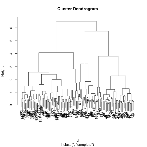
An illustrative example with the Iris data set
First obtaining the clustering with the Complete Linkage method (default)
data(iris)
d <- dist(scale(iris[,-5]))
h <- hclust(d)
Now cutting the dendrogram to form 3 clusters
cls <- cutree(h,3)
table(cls,iris$Species)
##
## cls setosa versicolor virginica
##   1     49          0         0
##   2      1         21         2
##   3      0         29        48
plot(h)
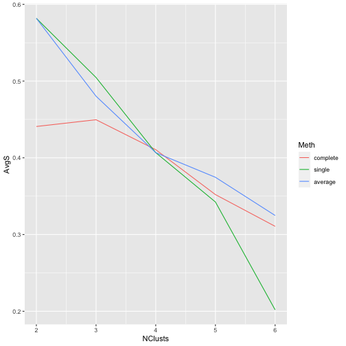
Silhouette coefficients to compare different alternatives
 library(cluster)
d <- dist(scale(iris[,-5]))
methds <- c('complete','single','average')
avgS <- matrix(NA,ncol=3,nrow=5,
               dimnames=list(2:6,methds))
for(k in 2:6) {
  for(m in seq_along(methds)) {
    h <- hclust(d,meth=methds[m])
    c <- cutree(h,k)
    s <- silhouette(c,d)
    avgS[k-1,m] <- mean(s[,3])
  }
}

library(reshape2)
dt <- melt(avgS)
colnames(dt) <- c("NClusts","Meth","AvgS")
library(ggplot2)
ggplot(dt,aes(x=NClusts,y=AvgS,color=Meth)) +
geom_line()
Divisive Hierarchical Clustering
These methods start by a single cluster and at each stage decide which cluster is split in two.
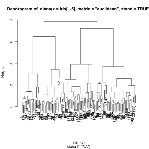
The DIANA method
- At each stage, choose the cluster with the largest diameter.
- The diameter of a cluster is the largest dissimilarity between any two of its observations
- To perform the group splitting the observation in that group with largest average dissimilarity to the other members of the group is selected
- Then all observations are allocated to either the cluster of this selected observation or to the "old" group (represented by its center), depending on which one is nearest
An illustrative example with the Iris data set
library(cluster)
di <- diana(iris[,-5],
            metric='euclidean',
            stand=TRUE)
table(cutree(di,3),iris$Species)
##
##     setosa versicolor virginica
##   1     50          0         0
##   2      0         11        33
##   3      0         39        17
pltree(di)
Hands-on Clustering
- Using the
irisdata set answer the following questions. - Store all the clustering results, and remember to ignore the target variable (
Species)!
Apply the k-means algorithm, and find the optimal number of clusters
Using the best \(k\), apply the PAM, CLARA, DBSCAN, FANNY, Agglomerative Hierarchical Clustering (
hclust()) and DIANA algorithmsCompare all results using the silhouette coefficient
